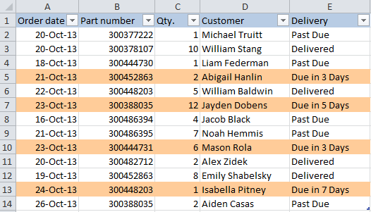
Say, you have a table of your company orders like this:

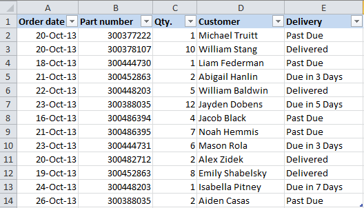
You may want to shade the rows in different colors based on the cell value in the Qty. column to see the most important orders at a glance. This can be easily done using Excel Conditional Formatting.

1. Start with selecting the cells the background color of which you want to change.
2. Create a new formatting rule by clicking Conditional Formatting > New Rule... on the Home tab.

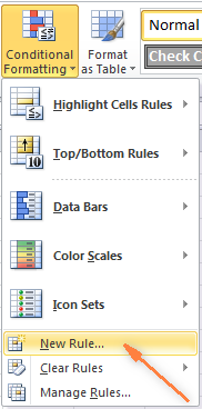
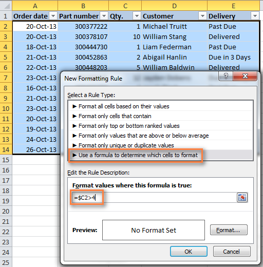
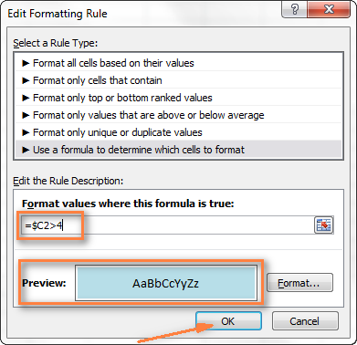
3. In the "New Formatting Rule" dialog window that opens, choose the option "Use a formula to determine which cells to format" and enter the following formula in the "Format values where this formula is true" field: =$C2>4

Instead of C2, you enter a cell that contains the value you want to check in your table and put the number you need instead of 4. And naturally, you can use the less (< ) or equality (=) sign so that your formulas will read =$C2<4 and =$C2=4, respectively.

Also, pay attention to the dollar sign $ before the cell's address, you need to use it to keep the column letter the same when the formula gets copied across the row. Actually, it is what makes the trick and applies formatting to the whole row based on a value in a given cell.

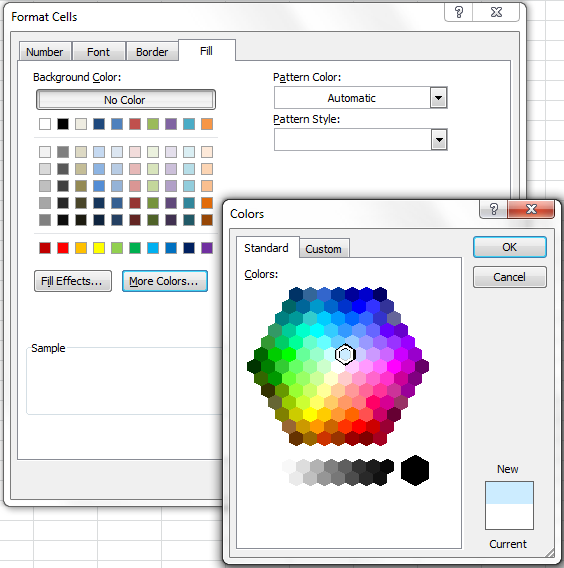
4. Click the "Format..." button and switch to Fill tab to choose the background color. If the default colors do not suffice, click the "More Colors..." button to pick the one to your liking, and then click OK twice.

You can also use any other formatting options, such as the font color or cells border on the other tabs of the Format Cells dialog.

4. The preview of your formatting rule will look similar to this:

5. If this is how you wanted it and you are happy with the color, click OK to see your new formatting in effect.

Now, if the value in the Qty. column is greater than 4, the entire rows in your Excel table will turn blue.

As you can see, changing the row's color based on a number in a single cell is pretty easy in Excel. Further on, you will find more formula examples and a couple of tips for more complex scenarios.

How to apply several rules with the priority you need

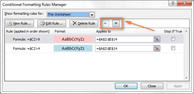
In the previous example, you may want to highlight the rows with different values in the Qty. column in different colors. For example, you can add a rule to shade the rows with quantity 10 or greater, say, in pink. In this case, use the formula =$C2>9, and after your second formatting rule is created, set the rules priority so that both of your rules will work.

1. On the Home tab, in the Styles group, click Conditional Formatting > Manage Rules... .

2. Choose "This worksheet" in the "Show formatting rules for" field. If you want to manage the rules that apply to your current selection only, choose "Current Selection".

3. Select the formatting rule you want to be applied first and move it to the top of the list using the arrows. The result should resemble this:

Click the OK button and the corresponding rows will immediately change their background color based on the cell values that you specified in both formulas.

How to change a row color based on a text value in a cell

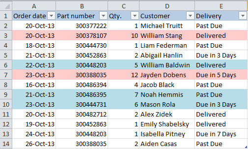
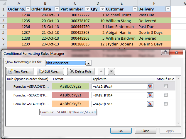
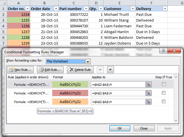
In our sample table, to make follow-up on orders easier, you can shade the rows based on the values in the Delivery column, so that:

If an order is "Due in X Days", the background color of such rows will turn orange;
If an item is "Delivered", the entire row will be colored in green;
If an order is "Past Due", the row will turn red.

Naturally, the row color will change if the order status gets updated.

While the formula from our first example could work for "Delivered" and "Past Due" (=$E2="Delivered" and =$E2="Past Due"), the task sounds a bit trickier for "Due in..." orders. As you see, different orders are due in 1, 3, 5 or more days and the above formula won't work because it is purposed for exact match.

In this case, you'd better use the =SEARCH formula like this =SEARCH("Due in", $E2)>0 that works for the partial match as well. In the formula, E2 is the address of the cell that you want to base your formatting on, the dollar sign ($) is used to apply the formula to the entire row, and >0 means that the formatting will be applied if the specified text ("Due in" in our case) is found.

Tip: If you use >0 in the above formula, it means that the row will be colored no matter where the specified value or text is located in the key cell. For example, the Delivery column (F) may contain the text "Urgent, Due in 6 Hours", and this row will be colored as well.

If you want to change the color of rows where the contents of the key cell starts with the indicated value or text, then you need to use =1 in the formula, e.g. =SEARCH("Due in", $E2)=1. However, be very careful when using this kind of formula and ensure that there are no leading spaces in the key column, otherwise you might rack your brain trying to figure out why the formula does not work :) You can use this free tool to find and remove leading and trailing spaces in your worksheets - Trim Spaces add-in for Excel.

Create three such rules following the steps from the first example, and you will have the below table, as the result:

How to change a cell's color based on a value of another cell

In fact, this is simply a variation of changing the background color of a row case. But instead of the whole table, you select a column or a range where you want to change the cells color and use the formulas described above.

For example, we could create three such rules to shade only the cells in the "Order number" column based on another cell value (values in the Delivery column).

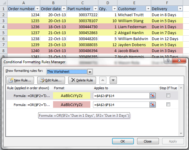
How to change a row's background color based on several conditions

If you want to shade the rows in the same color based on several values, then instead of creating several formatting rules you can use the =OR or =AND formulas to set several conditions.

For example, we can color the orders due in 1 and 3 days in the reddish color, and those that are due in 5 and 7 days in the yellow color. The formulas are as follow:

=OR($F2="Due in 1 Days", $F2="Due in 3 Days")


=OR($F2="Due in 5 Days", $F2="Due in 7 Days")

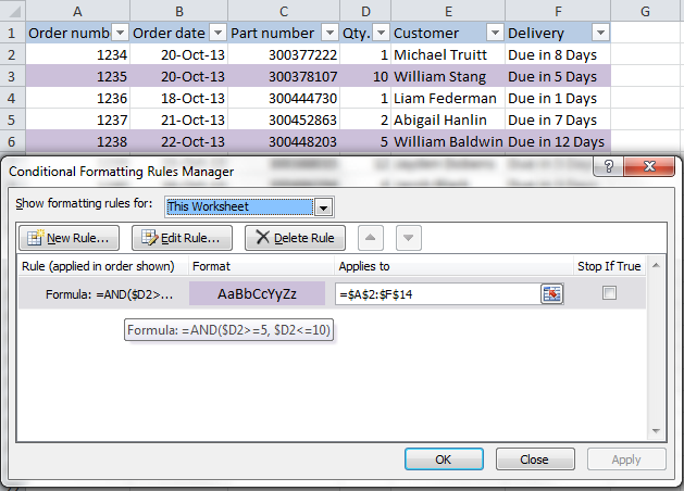
And you can use the =AND formula, say, to change the background color of rows with Qty. equal to or greater than 5 and equal to or less than 10: =AND($D2>=5, $D2< =10).

Naturally, you are not limited to using only 2 conditions in such formulas, you are free to use as many as you need, e.g. =OR($F2="Due in 1 Days", $F2="Due in 3 Days", $F2="Due in 5 Days") and so on.